ISSN 1884-0760
GRACE TECHNICAL REPORTS
Parallelizing Graph Structural Recursion
with BSP
Chong Li Le-Duc Tung Nhat-Tan Duong
Soichiro Hidaka Zhenjiang Hu
GRACE-TR 2015–02 Feb 2015
CENTER FOR GLOBAL RESEARCH IN
ADVANCED SOFTWARE SCIENCE AND ENGINEERING NATIONAL INSTITUTE OF INFORMATICS 2-1-2 HITOTSUBASHI, CHIYODA-KU, TOKYO, JAPAN
Parallelizing Graph Structural Recursion with BSP
Chong Li† Le-Duc Tung‡ Nhat-Tan Duong§
Soichiro Hidaka†‡ Zhenjiang Hu†‡
†National Institute of Informatics, Japan
‡Graduate University of Advanced Studies, Japan
§Hanoi University of Science and Technology, Vietnam
{chong, tung, hidaka, hu}@nii.ac.jp [email protected]
Abstract
The ever-increasing size of data today creates a critical need for scalable systems that can process large data efficiently. Graph structure can scale naturally to large datasets, as it does not require expensive join operations that are often needed by relational database querying. However, a complex query on a large graph is still very expensive in computa-tion. Moreover, optimizing algorithms of different queries is still needed to study case by case. Queries can be expressed by structural recursion like first-order logic extended with transitive closures. It gives us a new thinking that graph queries can be generalized in a structural-recursion way. Therefore, querying can be systematically evaluated in an efficient way by optimizing the structural recursion. In this paper, the structural recursion is first time implemented in parallel. A novel framework, based on Bulk Synchronous Parallelism (BSP), is thus proposed to evaluate large-graph queries. It provides a systematic way to deal with general graph queries. The implementation of the framework puts the structural recursion into practice and completes many unclear parts that cannot be covered by the the-ory. The performance evaluation shows that BSP can handle large-graph querying efficiently with a good scalability. The validation of our framework is an important step towards a systematic development of algorithms on large distributed graphs in which we can apply rules to automatically reasoning about programs.
Keywords: Structural recursion, Graph querying, Distributed computing, BSP
1
Introduction
The ever-increasing size of data today creates a critical need for scalable systems that can process large data efficiently. Graphs are useful to manage ad-hoc and evolving data like the World Wide Web [AJB99], social network [CSW05], biologic information [MV07], transportation system [APT04], etc. Moreover, graph structure can scale naturally to large datasets, as it does not require expensive join operations. However, a complex query on a large graph is still very expensive in computation. Efficient processing of large graphs becomes an open problem and more and more emergent in today’s big-data era.
Inspired by the complexity theory of PRAM model [GMR94] of parallel computers, Leslie Valiant [Val90] introduced the Bulk Synchronous Parallel (BSP) model. The BSP parallel al-gorithms can be designed and measured by taking into account not only the classical balance between time and parallel space (hence the number of processors) but also communication and synchronization. A BSP computation is a sequence of so-called supersteps. Each superstep combines asynchronous local computation with point-to-point communications that are coordi-nated by a global synchronization to ensure coherence and determinism. BSP provides a clear and sequential view of the parallel system, that is very efficient for designing complex parallel
algorithms. Inspired by BSP, Google [MAB+10] developed Pregel, a system for large-scale graph
processing. Several open-source Pregel-like systems [SYK+10, Ave11, SW13] were after proposed
too. These systems offer the possibility to design efficient parallel algorithms for large-graph processing. However, graph algorithms are still needed to be studied case by case. Implementing various algorithms is a very labour-intensive work. Moreover, there is no systematic guidance for designing efficient algorithms. Everything is still based on the experiences of developer. How to provide a systematic way to deal with large-graph queries is still an open problem.
Buneman et al. [BFS00] introduced a simple and powerful query language for graphs using structural recursion, which allows queries being expressed by first-order logic extended with transitive closures. It gives us a new thinking that graph queries can be generalized in a struc-tural recursive way. Therefore, instead of studying graph algorithms case by case, handling the structural recursion can systematically optimize large-graph querying. However, Buneman’s system “is adequate for small input graphs, e.g., graphs with at most 1000 nodes and 10000 edges, but it does not scale to large graphs with 10000 or more nodes”. There is still a big gap between structural recursion and parallel system. Parallel implementation of structural recur-sion does not exist. Previous researches discussed only the possibility of parallelizing structural recursion in theory briefly. We do not know how the evaluation works in parallel precisely in practice. Moreover, those theoretical proposals were never experimented. Implementing struc-tural recursion on a parallel platform becomes an essential challenge, that is an important step towards a systematic development of parallel algorithms on large graphs.
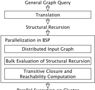
Figure 1: Overview of our parallel framework
recursion, and how such structural recursion can be evaluated efficiently in parallel.
This paper is organized as follow: Section 2 reviews the graph data model and the structural recursion proposed by Buneman et al. [BFS00]. Section 3 exploits the parallelizability of struc-tural recursion. In Section 4, we show how to implement efficient parallel strucstruc-tural recursion evaluation by using Bulk-Synchronous ML (BSML), a variant of CAML programming language developed by Loulergue et al. [Lou00]. The scalability of our implementation are studied in Section 5. The related work is discuss in Section 6 and the paper is concluded by Section 7.
Our contributions in the paper are: 1) studying the parallelizability of structural recur-sion with semantics inference rules; 2) developing the first parallel implementation of structural recursion evaluation, where we discover several optimizations and have improved the perfor-mance of evaluation; 3) validating the scalability of parallel evaluation of structural recursion, which encourages future researches on efficient structural recursion; and 4) proposing a general framework that can systematically process large-graph queries in an efficient way.
2
Graph Structural Recursion
Graph structural recursion, proposed by Buneman et al. [BFS00], is powerful with its simplicity and expressibility. In this section, we will review the graph structural recursion and its graph data model. A method for translating select-where queries into structural recursion is also presented in this section. Reader can, if he/she already knows Buneman et al.’s work on [BFS00], skip this section and go directly to next section.
2.1 Graph Data Model
Graphs we deal with in this paper isrooted,directed, andedge-labelled with no order on outgoing
edges. They are edge-labelled in the sense that all information is stored on labels of edges while labels of nodes serve only as a unique identifier without a particular meaning. Our graph data
model has two prominent features, markers andǫ-edges. Nodes may be marked with input and
output markers, which are used as an interface to connect them to other graphs. An ǫ-edge
represents a shortcut of two nodes, working like the ǫ-transition in an automaton.We useLabel
to denote the set of labels and Mto denote the set of markers.
Formally, a graphG, sometimes denoted byG(V,E,I,O), is a quadruple (V, E, I, O), whereV
is a set of nodes, E ⊆ V ×(Label∪ {ǫ})×V is a set of edges, I ⊆ M ×V is a set of pairs of
an input marker and the corresponding input node, and O⊆V × Mis a set of pairs of output
nodes and associated output markers. For each marker &x ∈ M, there is at most one node
v such that (&x, v) ∈ I. The node v is called an input node with marker &x and is denoted
by I(&x). Unlike input markers, more than one node can be marked with an identical output
marker. They are calledoutput nodes. Intuitively, input nodes are root nodes of the graph (we
allow a graph to have multiple root nodes, and for singly rooted graphs, we often use default marker & to indicate the root), while an output node can be seen as a “context-hole” of graphs
where an input node with the same marker will be plugged later. We write inMarker(G) to
denote the set of input markers and outMarker(G) to denote the set of output markers in a
graph G. In addition, we write label(ζ) to denote the label of the edge ζ.
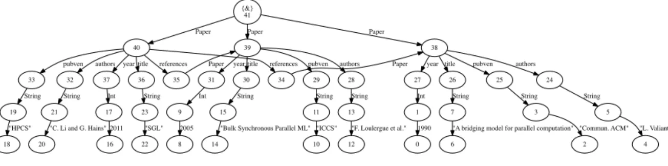
For instance, the graph in Figure 2 is denoted by (V, E, I, O) where,
V = {0 , 1 , 2 , 3 , 4 , . . . , 4 0 , 41}
E = {( 4 1 , Paper , 4 0 ) , ( 4 0 , pubven , 3 3 ) , ( 4 0 , r e f e r e n c e , 3 5 ) , ( 3 5 , Paper , 3 9 ) , ( 4 1 , Paper , 3 9 ) , ( 3 9 , t i t l e , 3 0 ) , . . . } I = {(& , 4 1 )}
O = { }.
{&} 41 40 Paper 39 Paper 38 Paper 37 year 36 title 35 references 34 references 33 pubven 32 authors 31 year 30 title 29 pubven 28 authors 27 year 26 title 25 pubven 24 authors 17 Int 23 String Paper Paper 19 String 21 String 9 Int 15 String 11 String 13 String 1 Int 7 String 3 String 5 String 22 "SGL" 20
"C. Li and G. Hains"
18 "HPCS"
16 2011
14
"Bulk Synchronous Parallel ML"
12
"F. Loulergue et al."
10 "ICCS"
8 2005
6
"A bridging model for parallel computation"
4 "L. Valiant" 2 "Commun. ACM" 0 1990
Figure 2: Graph of a digital library with 3 papers
G::= {} {single node graph}
| {a:G} {an edge pointing to a graph}
| G1∪G2 {graph union}
| &x:=G {label the root node with an input marker}
| &y {a node graph with an output marker}
| () {empty graph}
| G1⊕G2 {disjoint graph union}
| G1@G2 {append of two graphs}
| cycle(G) {graph with cycles}
As showing in Figure 3, {} constructs a root-only graph, {a : G} constructs a graph by
adding an edge with labela∈Label∪ {ǫ}pointing to the root of graphG, andG1∪G2 adds two
ǫ-edges from the new root to the roots ofG1andG2. Also, &x:=Gassociates an input marker,
&x, to the root node of G, &y constructs a graph with a single node marked with one output
marker &y, and () constructs an empty graph that has neither a node nor an edge. Further,
G1⊕G2 constructs a graph by using a componentwise (V, E, I andO) union. Operator∪differs
from ⊕ in that ∪unifies input nodes while ⊕ does not. Operator ⊕ requires input markers of
operands to be disjoint, while ∪ requires them to be identical. G1@G2 composes two graphs
vertically by connecting the output nodes of G1 with the corresponding input nodes of G2 with
ǫ-edges, and cycle(G) connects the output nodes with the input nodes of G to form cycles.
Newly created nodes have unique identifiers.
Figure 3: Graph Constructors
For example, the graph showing in Figure 2, that respects DBLP citation dataset schema
[TZY+08], can be constructed by using the above graph constructors:
&d l @
cy cle( (
&d l:={Paper :&p1, Paper :&p2, Paper :&p3}, &p1:={t i t l e :{S t r i n g : ”SGL”}, y e a r :{I n t : 2 0 1 1},
pubven :{S t r i n g : ”HPCS”}, r e f e r e n c e s :{Paper :&p2}, r e f e r e n c e s :{Paper :&p3} },
&p2:={t i t l e :{S t r i n g : ” Bulk Synchronous P a r a l l e l ML”}, y e a r :{I n t : 2 0 0 5}, a u t h o r s :{S t r i n g : ”F . L o u l e r g u e e t a l . ”},
pubven :{S t r i n g : ”ICCS”} },
&p3:={t i t l e :{S t r i n g : ”A b r i d g i n g model f o r p a r a l l e l computation ”}, y e a r :{I n t : 1 9 9 0},
a u t h o r s :{S t r i n g : ”L . V a l i a n t ”}, pubven :{S t r i n g : ”Commun . ACM”}} ) )
Here &dl@ which is used to declare that &dl@ is the root input marker (by the convention root
input marker is normally named &) and remove other input markers (e.g. &p1, &p2 and &p3
in our example) from the graph.
2.2 Graph Structural Recursion
Recursion is widely used by functional programming language for traversing dataset. However, different from list and tree structures, graph structure is much more general and complex, since it can include cyclic structure. A recursion without restriction might loop infinitely on such structure. That’s why we use a restricted form of recursion – structural recursion – to deal with the general structure. The restrictions of structural recursion are to ensure the termination of recursion.
A functionf on graphs is called a structural recursion if it is defined by the following
equa-tions:
f({}) = {}
f({$l: $g}) = e@f($g)
f($g1∪$g2) = f($g1)∪f($g2),
where the expression emay contain references to variables $l and $g (but no recursive calls to
f). Since the first and the third equations are common in all structural recursions, we write the
structural recursion simply as
f($db) =rec(λ($l,$g).e)($db)
whereecould be either graph variable (denoted by $g), conditional expression (if l=lthen e
else e, where l is either actual label or label variable $l), graph contructor (presented in
Sec-tion 2.1) or structural recursion expression.
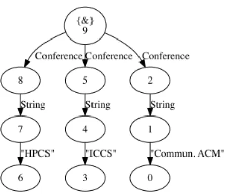
For example, for retrieving all papers’ conferences (pubven) in the graph of Figure 2, we can write the query in the structural recursion form as follows:
Q1 :=
rec(\ ($L,$f v 1) .
i f $L = Paper then
rec(\ ($L,$c) .
i f $L = pubven then
{C o n f e r e n c e : $c}
e l s e {} ) ($f v 1)
e l s e {} ) ($db)
This query firstly retrieves all subgraphs G1 that are under a Paper edge ({Paper : G1})
from the whole graph $db. Thus, each G1 contains all information of a paper. After that, it
retrieves subgraphs G2 that are under a pubven edge ({pubven : G2}) from each G1. So each
G2 is the conference information of a paper. At the end, we add a Conference edge before the
actual information of conference by replacing the pubven edge. Figure 4 shows the result of the
{&} 9
8
Conference
5 Conference
2 Conference
7 String
6 "HPCS"
4 String
3 "ICCS"
1 String
0
"Commun. ACM"
Figure 4: Result of Q1 for Figure 2
2.3 Translating Queries into Structural Recursion
Writing SQL-like queries is often easier than directly writing in the structural recursion form. For
example, Q1 that is used to retrieve all papers’ conference can be written in aselect. . .where. . .
surface syntax with pattern matching: Q2 :=
s e l e c t {C o n f e r e n c e :$c}
where { ∗. Paper . pubven :$c} in $db
For any regular path pattern, according to [Suc02], it can be translated into structural recursion by expressing first the regular expression as an automaton, and associating a function
with each state. For example, the regular expression ∗.P aper.pubvenin Q2 can be represented
by the automaton in Figure 5.
z1
z3
Paper z4
NOT(Paper) Paper
NOT(Paper OR pubven)
z2 pubven
Paper
NOT(Paper)
Paper NOT(Paper)
Figure 5: Automaton for Q2
The initial state is z1. If we meet a Paper-edge in z1 then it is changed to the state z3
otherwise to the statez4. The statesz2 andz4 are similar toz1, will be changed toz3 if meet
a Paper-edge otherwise to z4. The z3 is the state where we met aPaper-edge and waiting for a pubven-edge. Therefore its state will be remained when meet aPaper-edge but changes toz2
iff meet pubven. The statez2 is terminal state.
Based on the translated automaton, Q2 can be written like Q1 with mutually-recursive func-tion. Such mutually-recursive function can be translated into single-recursive function through tupling, where tuples of graphs are represented by disjoint union of graphs and projections of the
tuples as the idiom &z@ where &zis the component that are extracted by the tuples. Therefore,
Q3 :=
&z 1
@ rec(\ ($L,$c) .
i f $L = Paper
then (&z 4:=&z3, &z 3:=&z3, &z 2:=&z3, &z 1:=&z 3)
e l s e i f $L = pubven
then (&z 4:=&z4, &z 3:=(&z 2 U {C o n f e r e n c e :$c}) , &z 2:=&z4, &z 1:=&z 4)
e l s e (&z 4:=&z4, &z 3:=&z4, &z 2:=&z4, &z 1:=&z 4) ) ($db)
Now, we are able to write queries in a simple select. . .where. . . syntax with regular path
pattern. We know also how to translate a select-where query into structural recursion. In
addition, Hidaka et al. [HHI+12] proposed an optimization for rewriting structural recursion
queries based on markers analysis.
3
Parallelizability of Structural Recursion
We exploit, in this section, the parallelizability of structural recursion. The bulk semantics, which is one of solutions to evaluate structural recursion, is studied here by using inference rules. Select-where query is also studied to guarantee the parallelizability for more general case. At the end of this section, we show how to decompose a graph into a distributed one.
3.1 Bulk Semantics
There are several solutions to evaluate structural recursion by avoiding that recursive functions run into infinite loops on cyclic graph. For example, we can memorize all recursive calls then avoid entering infinite loops of recursion evaluation on graph. We can also do an inductive definition based on a constructor expression for the given data graph. However, such a definition can only be done under some technical restrictions.
Here we present a parallelizable solution called bulk semantics, which is also mentioned
briefly in [BFS00], but has never been implemented or experimented in parallel environment. The method applies the recursive function individually on all edges of the input graph. Therefore, all the possible results of the recursive functions are evaluated on each edge by using its label and subgraph as inputs of the function. We simply need to reconnect the above results according to the structural recursion. Moreover, each function will be applied only as many times as edges in the graph, and infinite loops are avoided.
LetG[a1 :G1] denotes that graph Gis composed of a1 :G1, and he, Gi →G′ denotes that
applying expressioneto graphGgets graphG′. Recursive evaluation of structural recursion
ex-pressionrec(λ($l,$g).e) applied to input graphGcan be summarized by the following inference
rules:
he, G[a1:G1]i@(he, G1[a2:G2]i@· · ·)→G′[G′0@(G′1@· · ·)]
he, G[a1 :G1]i@hrec(λ($l,$g).e), G1[a2:G2]i →G′[G′0@G′′]
hrec(λ($l,$g).e), G[a1:G1]i →G′
As defined in Section 2.2, the operation @ is associative. When the evaluation of expression
e depends only on a1 but not on Gi, we are able to apply body eindependently on every pair
(ai, Gi) in G where ai is the label of the edge and Gi is the graph that the edge is pointing
to. Once the the edges of Gwere evaluated with body e, then we can join the evaluated edges
with ǫ-edges (as in the @ constructor). Therefore, we obtain fully parallizable bulk semantics
for evaluating structural recursion:
he, G[a1:G1]i@he, G1[a2 :G2]i@· · · →G′[G′0@G′1@· · ·]
However, it also shows that there is a constraint for the body e: when applying the bulk
semantics, we do not have full information of the input graph Gany more, we shall use only the
information of the actual edge a.
3.2 Decomposed Query
Indeed, the current expression of structural recursion allows the bodyeuses the subgraphg. But
what will happen to bulk semantics? Here is an example for retrieving all P aper published in
2011 from the graph of Figure 2. SinceP aperis not used at the end of expression but in the
mid-dle, we need to split the regular expression ∗.P aper.year.Int.2011 to at least two parts (at most
five parts in our case: ∗,P aper,year,Intand 2011) in order to construct the select-where query:
s e l e c t {Paper2011 :$p}
where { ∗. Paper :$p} in $db, {year.Int: 2 0 1 1} in $p
In this query, the final result ($p) depends not only on the actual edge (where label $L =
P aper), but also on its subgraph where it needs to satisfy the expression year.Int: 2011.
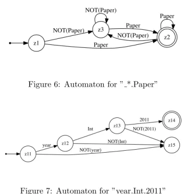
By decomposing the above query and translating them into two automata (Figure 6 and Figure 7), we can obtain the following embedding structural recursion:
&z 1
@ rec(\ ($L,$p) .
i f $L = Paper
then (&z3 := &z 2
U &z 1 1 @ rec(\ ($L,$f v 1) .
i f $L = y e a r
then {&z 1 1:=&z12, &z 1 2:=&z15, &z 1 3:=&z 1 5}
i f $L = I n t
then {&z 1 1:=&z15, &z 1 2:=&z13, &z 1 3:= $z15}
i f $L = 2011
then {&z 1 1:=&z15, &z 1 2:=&z15, &z 1 3:=&z 1 4 U {Paper2011 : $p}}
e l s e {&z 1 1:=&z15, &z 1 2:=&z15, &z 1 3:=&z 1 5}) ($p) ,
&z 2 := &z 2
U &z 1 1 @ rec(\ ($L,$f v 1) .
i f $L = y e a r
then {&z 1 1:=&z12, &z 1 2:=&z15, &z 1 3:=&z 1 5}
i f $L = I n t
then {&z 1 1:=&z15, &z 1 2:=&z13, &z 1 3:= $z15}
i f $L = 2011
then {&z 1 1:=&z15, &z 1 2:=&z15, &z 1 3:=&z 1 4 U {Paper2011 : $p}}
e l s e {&z 1 1:=&z15, &z 1 2:=&z15, &z 1 3:=&z 1 5}) ($p) ,
&z 1 := &z 2
U &z 1 1 @ rec(\ ($L,$f v 1) .
i f $L = y e a r
then {&z 1 1:=&z12, &z 1 2:=&z15, &z 1 3:=&z 1 5}
i f $L = I n t
then {&z 1 1:=&z15, &z 1 2:=&z13, &z 1 3:= $z15}
i f $L = 2011
then {&z 1 1:=&z15, &z 1 2:=&z15, &z 1 3:=&z 1 4 U {Paper2011 : $p}}
e l s e {&z 1 1:=&z15, &z 1 2:=&z15, &z 1 3:=&z 1 5}) ($p) ,
e l s e (&z3 := &z3 , &z 2 := &z3 , &z 1 := &z3 ) ) ($db)
The inference rules of embedding structural recursion thus become:
(heg, Gi ⊙ hea, Gi)@(heg, G1i ⊙ hea, G1i)@· · · →G′[G′0[Gg0⊙Ga0]@G′1[Gg1⊙Ga1]@· · ·]
he, G[a1:G1]i@he, G1[a2 :G2]i@· · · →G′[G′0@G′1@· · ·]
z1
z3 NOT(Paper)
z2 Paper
NOT(Paper)
Paper NOT(Paper)
Paper
Figure 6: Automaton for ” *.Paper”
z11
z12
year z15
NOT(year) z13 Int
NOT(Int)
z14 2011
NOT(2011)
Figure 7: Automaton for ”year.Int.2011”
where eg is the inner structural recursion rec(λ($l,$g).einner) using the same bulk semantics
inference rules,eais partial expression ofeexcluding the inner structural recursion, and⊙is the
relation between eg and ea. Therefore, an embedding structural recursion is still parallelizable
by using divide-and-conquer approach. However, information of graph need to be replicated recursively that will increase heavily communication cost in a distribute-memory environment.
There are also other cases of non-decomposed query. Since our select-where queries are using regular expression or its composition, We can always split queries down to decomposed ones in order to maintain the parallelizability of the querying. To have as less as possible
the decomposed parts of a query Q(g) or Q(l, g), where g is an input graph variable and l, if
needed, is an input label variable, in order to have better performance, we here borrow six forms from [Suc02]. These forms are originally to restrict select-where queries on tree structure. A decomposed select-where subquery must be in one of these forms:
1. g;
2. {};
3. {a:Q1(l, g)} whereais either l or a label constant;
4. Q1(l, g)∪Q2(l, g);
5. selectQ1(g1) where {R:g1} ing;
6. selectQ1(l1, g1) where{R:l1 :g1} ing, P(l1);
where P(l1) is a unary predicate, R is regular expression,Q1 and Q2 are themselves restricted
select-where queries with variable marked accordingly. Therefore, if a query selectE whereP
indbcan be translated into one single structural recursion union with an input marker, which is
used to indicate the initial state (e.g. &z1 in the structural recursion query on Page 8), then P
may introduce only one graph variable gand, if needed, a label variableloccurring right before
g.
Letf(G) be a function for querying the graph G,f has decomposability iff:
{&dl} 19 18 Paper 17 {&p2} Paper 16 {&p3} Paper 15 year 14 title 13 references 12 references 11 pubven 10 authors 3 Int 9 String 1 {&p2} Paper 0 {&p3} Paper 5 String 7 String 8 "SGL" 6 "C. Li and G. Hains" 4
"HPCS" 2
2011
(a) Partition 1
{&p2} 12 11 year 10 title 9 pubven 8 authors 1 Int 7 String 3 String 5 String 6
"Bulk Synchronous Parallel ML" 4
"F. Loulergue et al." 2
"ICCS" 0
2005
(b) Partition 2
{&p3} 12 11 year 10 title 9 pubven 8 authors 1 Int 7 String 3 String 5 String 6
"A bridging model for parallel computation"
4 "L. Valiant" 2 "Commun. ACM" 0 1990
(c) Partition 3
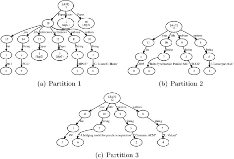
Figure 8: Distributed Graph with 3 Partitions
• ∀G1, G2|f(G1⊕G2) =f(G1)⊕f(G2).
It provides the possibility to evaluate queries in parallel by decomposing the database.
3.3 Distributed Graph
In this subsection, we will study how to decompose a graph data into distributed one by extend-ing the basic graph data usextend-ing some special markers. Therefore, a very large graph data could be split into several partitions and distributed to computer cluster. These special markers are
called cross links. Similar to [Suc02], cross links are used to split nodes in different partitions.
Across link is an edgeu→vlabelled withǫfor whichuandvare stored on different partitions.
Therefore, a node acan be split into two nodes aand a′ with a cross link a→ǫa′.
In practice, we use input markers and output markers with the same name to describe cross
links instead of creating real ǫ-edges. For example, Figure 8 is a distributed graph1 with 3
partitions that contains the same information of the graph of Figure 2. The nodes 38 and 39 of Figure 2 are split here to create cross links that bridge partitions with input and output
markers. Splitting the node under Paper is not mandatory, any node of the graph can be split
to different partitions by using cross link.
In general, a distributed graphGcan be expressed as:
&z1@cyclez(G1⊕ · · · ⊕Gp)
where z is a set of input markers z = {&z1, . . . ,&zn} whose size is the number of cross links
plus one, &z1 is the root input marker, and G1, . . . , Gp are the subgraphs on p partitions.
For example, &dl@cycle(db1⊕db2⊕db3) is equal to the graph of Figure 2, where db1,db2
and db3 are the 3 partitions of the distributed graph shown in Figure 8:
db1:=
&d l @
cy cle( (
&d l:={Paper :&p1, Paper :&p2, Paper :&p3}, &p1:={t i t l e :{S t r i n g : ”SGL”}, y e a r :{I n t : 2 0 1 1},
a u t h o r s :{S t r i n g : ”C . L i and G. Hains ”}, pubven :{S t r i n g : ”HPCS”},
1
r e f e r e n c e s :{Paper :&p2}, r e f e r e n c e s :{Paper :&p3}} ) )
db2:=
cyc le( (
&p2:={t i t l e :{S t r i n g : ” Bulk Synchronous P a r a l l e l ML”}, y e a r :{I n t : 2 0 0 5}, a u t h o r s :{S t r i n g : ”F . L o u l e r g u e e t a l . ”},
pubven :{S t r i n g : ”ICCS”}} ) )
db3:=
cyc le( (
&p3:={t i t l e :{S t r i n g : ”A b r i d g i n g model f o r p a r a l l e l computation ”}, y e a r :{I n t : 1 9 9 0},
a u t h o r s :{S t r i n g : ”L . V a l i a n t ”}, pubven :{S t r i n g : ”Commun . ACM”}} ) )
Therefore, for a decomposed function f(G), with which we know [Suc02] f(cycle(G)) =
cycle(f(G)), can be applied on a distributed graphG(e.g. the one in Figure 2), then we obtain
f(&z1)@cyclez(f(G1)⊕ · · · ⊕f(Gp))
Bulk semantics of structural recursion on distributed graph work also well in parallel:
(he, G[a11 :G11]i@· · ·)⊕ · · · ⊕(he, G[a1p :G1p]i@· · ·)→G′[G′
1[G01′@· · ·]⊕ · · · ⊕G′p[G0p′@· · ·]]
hrec(λ($l,$g).e), G1i ⊕ · · · ⊕ hrec(λ($l,$g).e), Gpi →G′[G′1⊕ · · · ⊕G′p]
hrec(λ($l,$g).e), G[G1⊕ · · · ⊕Gp]i →G′[G′1⊕ · · · ⊕G′p]
We are now able to store very large graph in a distributed environment by using cross links. We will describe the implementation of the parallel framework for structural recursion in next section.
4
Structural Recursion over BSP
GRoundTram2 [HHI+11], which is a system to build bidirectional transformation between two
models (graphs), uses the basic graph data model presented in Section 2. In this section, we will use BSML to extend the sequential structural recursion of GRoundTram to parallel one. The parallel bulk semantics is first time implemented in practice. Thanks to the clarity of BSP model, the performance of our parallel implementation can be understood easily.
4.1 Bulk-Synchronous Parallelism
4.1.1 BSP Model
The Bulk-Synchronous Parallel (BSP) model is a parallel programming model introduced by Leslie Valiant [Val90]. It offers a high degree of abstraction like PRAM models [FW78] and yet allows portable and predictable performance on a wide variety of multi-processor architectures [SHM97]. The major difference between BSP and PRAM is that the local computations of BSP are asynchronous, and the cost of inter-processor communications in BSP is not neglected.
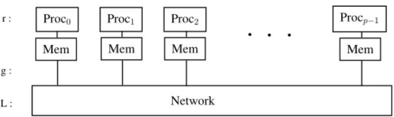
A BSP computer contains:
• a homogeneous set of uniform processor-memory pairs;
• a communication network allowing inter-processor delivery of messages;
• and a global synchronization unit which executes collective requests for a synchronization
Proc0 Proc1 Proc2 Procp−1
Network
b b b
Mem Mem Mem Mem
r :
g :
L :
Figure 9: A BSP computer
A wide range of actual architectures can be simulated by a BSP computer, including share-memory machines (via BSPRAM [Tis96]). Moreover, the synchronization unit is very rarely a hardware but rather a software event [HS98]. Supercomputers and clusters of PCs can be modelled as BSP computers.
A BSP program is executed as a sequence of supersteps (Figure 10), each one is divided
into (at most) three successive and logically disjoint phases:
1. In the first phase, each processor uses its local data (only) to perform sequential compu-tations and to request data transfers to/from other nodes.
2. In the second phase, the network delivers the requested data transfers.
3. And in the third phase, a global synchronization barrier occurs, making the transferred data available for the next superstep.
P1 P2 P3 Pp
Synchronization barrier
Synchronization barrier
BSP superstep
Figure 10: A BSP superstep
The performance of the BSP machine is characterised by 4 parameters:
• the local processing speed r;
• the number of processor-memory pairs p;
• the time Lrequired for a global synchronization (barrier);
• and the time g for collectively delivering a 1-relation communication phase where every
processor receives/sends at most one word.
The network can deliver anh-relation (every processor receives/sends at most h words) in
time g×h. To accurately estimate the execution time of a BSP program these 4 parameters
could be easily benchmarked [Bis04].
2Source codes of GRoundTram are available online at
The execution time (cost) of a superstepsis the sum of the maximum local processing time, the data delivery and the global synchronisation times. It is expressed by the following formula:
Cost(s) = max
0≤i≤p{w
s
i}+ max
0≤i≤p{h
s
i ×g}+L
wherewisis the local processing time on processoriduring supersteps, andhis= max{hsi+, hsi−}
wherehs
i+ (resp. hsi−) is the number of words transmitted (resp. received) by processoriduring
superstep s.
The total cost of a BSP program composed ofS supersteps is PSCost(s). It is, therefore,
the sum of three terms:
W +H×g+S×L
where W =PSmaxi{wsi}and H =
P
Smaxi{hsi}.
4.1.2 BSML Programming
BSML3 [LGB05] developed at Universit´e d’Orl´eans and Universit´e Paris-12 (now called
Uni-versit´e Paris-Est Cr´eteil or UPEC) is a library for OCaml4 implementing partially the Bulk
Synchronous Parallel ML language [Gav05]. There is in BSML an abstract polymorphic type
α par which represents the type ofp-wide parallel vectors of values of type α, one per process.
It is very different from usual SPMD programming where messages and processes are explicit, and programs may be non-deterministic or may contain deadlocks. In fact a large subset of BSML parallel programs are purely functional. The core BSML library is based on the following primitives:
mkpar : (int→α)→α par
proj : α par→(int→α)
apply : (α →β)par →α par→β par
put : (int→α)par →(int→α) par
The semantics of BSML primitives is described by the use of parallel values. Parallel value
<x0, x1,. . ., xp−1> represents a set of local values of a given type, such that xi is stored on
processor iand pis the number of processors.
In BSML,mkparis the parallel constructor: mkpar f computes the value<f 0,f 1,. . .,f
(p−1)>. proj is the parallel destructor: proj <x0,x1,. . .,xp−1>computes a functionf such
that (f i) =xi. applyis the asynchronous parallel transformer: apply <f0,f1,. . .,fp−1> <x0,
x1,. . .,xp−1>computes <f0x0,f1x1,. . .,fp−1xp−1>.
Finally, put is the synchronous (communicating) parallel transformer: put <g0, g1,. . .,
gp−1>computes a parallel vector of functions that contains the transported messages that were
specified by the gi. The input local functions are used to specify the outgoing messages thus:
gi j is the value that processoriwishes to send to processorj. The result of applying put is a
parallel vector of functions dual to the gi: they specify which value was received from a given
distant processor.
The execution of mkparis purely local and so is the execution of theapplyprimitive. The
execution of proj uses an all-to-all communication and the execution of put is a general BSP
communication (any processor-processor relation can be implemented with it). Recently, Li
and Hains [LH14] proposed a new function named gpsto simplify the put function. This new
function separates the meta data and actual data, and provides a sequential view to program parallel communication.
3
Bulk Synchronous Parallel ML.http://traclifo.univ-orleans.fr/BSML/
4Objective Caml.
4.2 Parallelizing Input and Output
Our parallel implementation takes an input graph and a structural recursion query, and produces an output graph. Different from GRoundTram, the input and output graphs are both distributed using cross links presented in Section 3.3 and stored in different files. Therefore, large graphs can be efficiently loaded and saved in parallel by different processor with parallel I/O.
Naturally, a large input graph is always split in advance by database administrator and distributed on different nodes of a parallel machine. In our implementation, a distributed input
graph with p partitions (like Figure 8 which is distributed into 3 partitions) is stored inp files.
Therefore, we have distributed input graph
G1⊕G2⊕ · · · ⊕Gp
where Gi(i= 1. . . p) is a local subgraph in partition i.
We want each partition is handled by a compute node (i.e. processor-memory pairs in BSP
model). So BSML function mkparis used to load the distributed graph into system:
mkpar(funpid→load subgraph Gpid+1)
Therefore, partitionsG1, G2, . . . , Gp are mapped to processorspid= 0, pid= 1, . . . , pid=p−1:
< G1, G2, . . . , Gp > .
In fact, the node IDs in each partition are used locally. But after loading the graph, node ID will be combined with partition ID for distinguishing nodes that have the same local ID from different partitions. This step does not produce any communication cost, and the computation costs max0≤i≤p{load subgraph Gi}.
The other input argument is a structural recursion queryQ. Here we study only decomposed
queries. If the input query is a more complex one, we shall decompose it by using the technique presented in Section 3.2. Since the bulk semantics will apply the structural recursion on each
edge, we also need to replicate Qin order to map it to each processor:
mkpar(funpid→Q)
Then we obtain
< Q, Q, . . . , Q > .
Since the size of the input query Q is tiny comparing to the input graph, communication cost
and computation cost here for distributing Qcan be neglected.
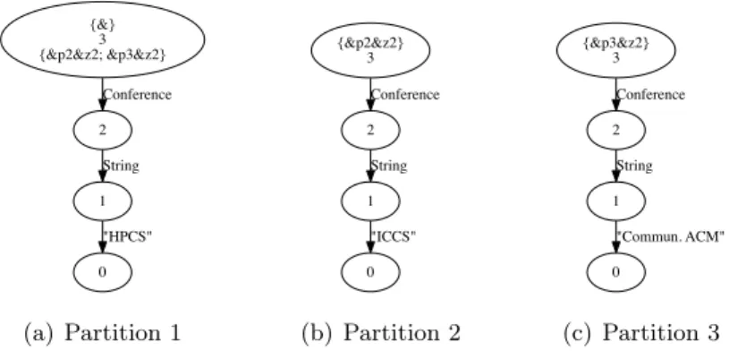
We keep the output graph also distributed, because 1) the result could be very big, for example if we want to retrieve the whole database; 2) communication cost can be reduced, since we do not need to move nodes and edges from one partition to another partition. Figure 11 is the distributed output graph created by applying Q3 on the distributed input graph of Figure 8. We will explain how to evaluate Q3 in the following sections. Therefore, the final result will be in the form of
< G′1, G′2, . . . , G′p >
A non-distributed final result could also be constructed with these G′i(i= 1. . . p):
{&} 3 {&p2&z2; &p3&z2}
2 Conference
1 String
0 "HPCS"
(a) Partition 1
{&p2&z2} 3
2 Conference
1 String
0 "ICCS"
(b) Partition 2
{&p3&z2} 3
2 Conference
1 String
0
"Commun. ACM"
(c) Partition 3
Figure 11: Result of Figure 8 for Q3
4.3 Parallelizing Bulk Evaluation
The form of our input structural recursion is like &z1@rec(λ($l,$g).e), whereeis the recursion
body, and &z1 is the root input marker. Since the bulk semantics focus only on the structural
recursion evaluation, before evaluating the query, we split it into 2 parts:
rc=rec(λ($l,$g).e)
and
mk= &z1@rc.
The bulk evaluation only take care of rc. mk will only be used later by the epsilon elimination
step presented in next subsection. This optimization technique is coherent to Buneman et al.’s sequential implementation [BFS00].
According to the bulk semantics, applying Qrc to (G1⊕ · · · ⊕Gp) is equal to applyingQrc
to eachGi(i= 1. . . p) individual then union the evaluated subgraphs by using⊕. Therefore, we
can evaluate our distributed input graph in parallel by using the BSML function:
apply < Qrc, Qrc, . . . , Qrc> < G1, G2, . . . , Gp >
This step is equal to
Qrc(G1)⊕Qrc(G2)⊕ · · · ⊕Qrc(Gp)
We obtain, after this step, the bulk-evaluated distributed graph
< G′1, G′2, . . . , G′p > .
This step costs max0≤i≤p{Qrc(Gi)}for computation and 0 for communication.
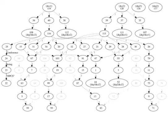
For example, Figure 12 is the result subgraphs of partition 1 of the distributed graph in
Figure 2 after applying Q3 using bulk semantics5. In the figure, ǫ-edges are denoted by the
dotted lines, and the currently unreachable nodes that have no input marker are in gray color.
4.4 Optimizing Epsilon Elimination
After bulk evaluation, the result distributed graph contains many edges and nodes that we do not need (cf. Figure 12). For obtaining a clean clear final result (like the one in Figure 11), we
need to 1) glue nodes by removing theǫ-edges, and 2) remove the nodes that cannot be reached
by the root input marker described with mk.
The easiest-to-design way to obtain the final result is to gather all evaluated subgraphs, then
rebuild ǫ-edge of cross-links by matching the input and output markers, and at the end fetch
5
Figure 12: Partition 1 of Figure 8 after bulk evaluation
the reachable part of the large assembled graph. However, the intermediate result after bulk semantics evaluation is very big (c.f. Figure 12), often bigger than the original graph. Gathering and centralizing such big data is very communication-intensive and not realistic.
Since the size of final result could be very big too, our implementation keeps the final result in a distributive way. To avoid to create unnecessary communication cost, the result edges shall stay in the same partition as where the original edges were. We propose here a recursive
functionreachability (Figure 13) to compute all reachable elements (nodes, edges, input markers
and output markers) from source sub-graph. This function takes 4 input arguments: 1. local
source sub-graph, 2. map of (node→outgoing edges) according to the local source sub-graph , 3.
global reachable output markers accumulator (initialized with root input marker), 4. reachable graph elements accumulator (initialized to empty); and produces a quadruple of nodes, edges, input markers and output markers to create the reachable subgraph(s) of each partition. The function is processed as follows:
1. locally compute the reachable elements of local graph according to the markers from marker accumulator (line 2), the result is a tuple of graph elements accumulator and output marker accumulator;
2. separate the graph elements accumulator and the marker accumulator (lines 3 - 4);
3. gather all cumulated reachable markers and broadcast to all processors (line 5);
4. check if there are new found output markers that we did not compute (line 6);
5. if there is no more new untested marker, then we stop the recursion, otherwise we make the recursive call (lines 7 - 8).
In the reachability function, parfun : (α → β) → α par → β par is equal to fun f a →
apply (mkpar(fun pid → f)) a; parfun2 : (α → β → γ) → α par → β par → γ par is
equal to fun f a b → apply (apply (mkpar(fun pid → f)) a) b; parfun4 : (α → β →
γ → δ → ǫ) → α par → β par → γ par → δ par → ǫ par is same as parfun and parfun2
but with 4 input parameters instead; and fold direct : (α → α → α) → α par → α par is a
1l e t rec r e a c h a b i l i t y = fun s o u r c e G r a p h s outgoEdgeMap markersCumul graphEltsCumul
−>
2 l e t locCumulReached = p a r f u n 4 l o c a l R e a c h a b l e s o u r c e G r a p h s outgoEdgeMap
markersCumul graphEltsCumul in
3 l e t r e a c h e d G r a p h E l t s = p a r f u n (fun ( g ,m) −> g ) locCumulReached in 4 l e t r e a c h e d M a r k e r s = p a r f u n (fun ( g ,m) −> m) locCumulReached in 5 l e t r e a c h e d M a r k e r s = f o l d d i r e c t S e t o f M a r k e r . union r e a c h e d M a r k e r s in 6 l e t stopCond = p a r f u n 2 S e t o f M a r k e r . e q u a l markersCumul r e a c h e d M a r k e r s in 7 i f (p r o j stopCond 0 ) then r e a c h e d G r a p h E l t s
8 e l s e r e a c h a b i l i t y s o u r c e G r a p h s outgoEdgeMap r e a c h e d M a r k e r s r e a c h e d G r a p h E l t s
Figure 13: BSML code ofcompute function
value <v0, v1,. . ., vp−1>, then produces a parallel value <s0, s1,. . ., sp−1> where s0 = · · · = sp−1 =v0⊕ · · · ⊕vp−1 and p is the number of processors. Communication cost offold direct is
(p−1)×n×g+l, wherenis the average size of valuesvi,gis the cost that one processor transfers
a word to another processor, andlis the cost of synchronizing all processors. The initial values
of markersCumul is a set with one element which is the root input marker (left side ofmk, e.g.
&z1 of &z1@rc); and the value of sourceGraphs is the bulk-evaluated distributed graph <G′1,
G′
2,. . .,G′p>but in quadruple form (nodes, edges, input markers and output markers).
Removingǫ-edges is the most expensive computation. We need to compute transitive closure
for all ǫ-edges, and the transitive closure computation is very costly. The ǫ-edge removing is
processed by adding new edges that glue nodes betweenǫ-edges to skip theǫ-closure. Removing
ǫ-edges does not require information for neighbour partition, Our implementation uses simply
apply to perform this step in parallel.
Sequential GRoundTram first perform the ǫ-edges elimination then the reachability.
How-ever, after our experiments and performance analysis, the optimal way, both for sequential and parallel computing, is to eliminate the unreachable parts first, then perform the epsilon elimi-nation only on the reachable parts. Therefore, in our implementation, after the bulk evaluation,
we firstly compute the reachability and remove the unreachable parts, then remove the ǫ-edges
in parallel for each cleaned partition.
5
Evaluation
The implementation of structural recursion evaluation querying graphs in parallel is experi-mented and will be discussed in the section.
5.1 Environment
The parallel machine used for the experiments is a computer cluster at the International Institute
for Computational Science and Engineering, HUST6. This supercomputer consists of 1 rack with
15 compute nodes, where we use 5 of compute nodes to evaluate the efficiency and scalability of our parallel implementation. Each compute node is configured with:
• 4 Intel Xeon E5-2679 CPUs @ 2.6GHz (16 cores per node)
• 32 GB RAM @ 1600 MHz and 300 GB HDD
• FDR 56Gbs Infiniband
• CentOS 6.5 64-bit
The following software are also deployed on the cluster, and loaded into the environment of each compute node:
6
• OpenMPI version 1.8
• Objective Caml (OCaml) v 4.0.2
• Bulk Synchronous Parallel ML (BSML) library v 0.4+beta2
The BSML library, which is based on OCaml, supports both TCP and MPI in parallel mode. Here, BSML uses OpenMPI for its communication.
5.2 Datasets
Datasets to be queried shall be a rooted, directed, and edge-labelled graph distributed into partitions and connected via cross links. All information is stored on label of edges, while label of nodes has no particular meaning but serve only as a unique identifier. This distributed graph can be in any shape including cyclic graph and tree. Since in bulk semantics a graph is evaluated edge by edge individually, the shape of graph does not have impact to the performance of evaluation, but it could indeed affect in some case the performance of epsilon-closure computation.
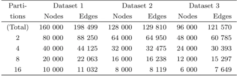
We created a generator to produce distributed random graphs. Our generated distributed random graph is cyclic, and each edge is labelled with a randomly chosen letter which is one of 26 Latin letters between “a” to “z”. Three random datasets were generated (Table 1). They were split into 2, 4 8 and 16 partitions in equilibrium.
Table 1: Sizes of graphs for experiments
Parti- Dataset 1 Dataset 2 Dataset 3
tions Nodes Edges Nodes Edges Nodes Edges
(Total) 160 000 198 499 128 000 129 810 96 000 121 570
2 80 000 88 250 64 000 64 950 48 000 60 785
4 40 000 44 125 32 000 32 475 24 000 30 393
8 20 000 22 063 16 000 16 238 12 000 15 297
16 10 000 11 032 8 000 8 119 6 000 7 649
5.3 Queries
Queries can be written in select. . .where. . . form with regular path patterns then translated
into structural recursion as explained in Section 2.3. Here, we write queries directly in struc-tural recursion form for having a clearer understanding. All queries described below are used for retrieving information from our distributed random graphs described in previous section. Evaluation of the queries is discussed in next section.
• Query 4: Replace all vowels (a, e, i, o, u) by 1,2,3,4,5 respectively, and keep the conso-nants (other than vowels) as they are.
&z 1 @
rec(\ ($l,$g) .
i f $l = a then &z 1:={ 1:&z 1}
e l s e i f $l = e then &z 1:={ 2:&z 1}
e l s e i f $l = i then &z 1:={ 3:&z 1}
e l s e i f $l = o then &z 1:={ 4:&z 1}
e l s e i f $l = u then &z 1:={ 5:&z 1}
e l s e &z 1:={$l:&z 1} ) ($db)
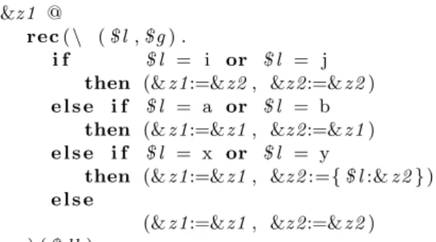
• Query 5: Select allx and y that are reachable by anior a j no matter after how many
steps, but in between of the path we could not have a or b. If there are more than one
path from anito an xand at least one of these paths does not contain aorbthen thisx
&z 1 @
rec(\ ($l,$g) .
i f $l = i or $l = j
then (&z 1:=&z2, &z 2:=&z 2)
e l s e i f $l = a or $l = b
then (&z 1:=&z1, &z 2:=&z 1)
e l s e i f $l = x or $l = y
then (&z 1:=&z1, &z 2:={$l:&z 2})
e l s e
(&z 1:=&z1, &z 2:=&z 2) ) ($db)
This query can be considered as an automaton with 3 states: initial state where we did
not reach any i or j; active state after reaching an i or j where it can be back to initial
state if touch aaorb; and the final state when reach x ory. However, the final state has
the same conditions as the active state: 1) back to the initial state if touch a a or b 2)
maintain the state otherwise. That’s why we merged these two states into one.
5.4 Experiments
We experimented both Query 4 and Query 5 on the computer cluster described in Section 5.1. First, we fix the size of querying distributed graph and vary the number of processors. The size of subgraph in each partition will be decreased when the number of processors increases for keeping the size of the whole distributed graph consistent. After that, we fix the number of processors and vary the size of distributed graph. In this step, when the size of distributed graph increases, the size of each partition’s sug-graph increases too. Meanwhile, the number of cross links increases in the same time, since more nodes are spilt into different partitions. During our experiments, each processor processes one partition data. For each experiment, the execution times of bulk evaluation, reachability and epsilon elimination are measured separately.
�� ���� ����� ����� ����� ����� ����� ����� ����� ����� ����� � � � �� ����� �� ��� � �� ���� ��� ��� � ������������������������ ��������������� ������������ ���������������
(a) Query 4 on dataset 1
�� ���� ����� ����� ����� ����� ����� � � � �� ����� �� ��� � �� ���� ��� ��� � ������������������������ ��������������� ������������ ���������������
(b) Query 4 on dataset 2
�� ���� ���� ���� ���� ����� ����� ����� ����� ����� � � � �� ����� �� ��� � �� ���� ��� ��� � ������������������������ ��������������� ������������ ���������������
(c) Query 4 on dataset 3
�� ��� ��� ��� ��� ��� ��� ��� ��� �������� �������� �������� ����� �� ��� � �� ���� ��� ��� � �������� ��������������� ������������ ���������������
(d) Query 5 with 16 partitions
Figure 14: Execution time of experiments
Query 4 is equivalent to an automaton with only 1 state. During bulk evaluation, each edge compare its label, then either relabel it if it is a vowel, or keep the consonant otherwise.
for this query. Since no edge is deleted, there is no long and deep chainedǫ-edges but just only
1-stepǫ-edges created during bulk evaluation. The execution time of reachability computation,
which is used to clean the unreachable parts, is very short too for this query. As we know, this “automaton” has only 1 state, the number of candidate edges were therefore not multiplied. We need just to pass one and only one time for each edge and the number of edges is just same as the original graph. Figure 14 (a) (b) and (c) show the execution time of Query 4 by varying the number of processors (partitions) and the size of querying graph.
z1 _
z2 i | j
a | b _ x | y -> mark it
Figure 15: Automaton equivalent to Query 5
Query 5 fetches only the reachablex-edges andy-edges according to the conditions, all other
edges will be contracted. The reachability computation is doubled because there is two states so each edge becomes two edges depending on states of automaton (Figure 15). In fact, during bulk evaluation, all edges are multiplied according to the number of state that the equivalent automaton has. Therefore a complex query will be very expensive. The epsilon elimination here is extremely expensive, because the transitive closure computation is very expensive by its
nature. Furthermore, there are many long chainedǫ-edges and the number of edges were already
multiplied. That’s why, the sequential implementation of structural recursion evaluation
pro-posed by Hidaka et al. [HHI+11] cannot handle epsilon elimination for large graphs. Our parallel
implementation processes first the reachability computation then the epsilon elimination after. It optimized significantly the performance. Moreover, the parallel reachability computation is also optimized by using accumulators and collective communication via MPI. That’s why we can obtain a linear speedup, and it is even faster than other implementation in sequential without using parallelism features. Figure 14 (d) shows the execution time of Query 5 in varying the size of graph.
The results of experiments confirm the theoretical proposals and assumptions. Our imple-mentation have linear speedup and sometimes super linear speedup for some complex queries since the reachability computation and epsilon elimination are optimized for both sequential computing and parallel computing. The validation of our implementation is an important step towards a systematic development of algorithms for large graph querying. More research can therefore be established based on this gratified results.
6
Related Work
Evaluating regular path queries on distributed, rooted, edge-labelled directed graphs were stud-ied by Dan Suciu [Suc02]. Theoretically, algorithms in [Suc02] are efficient in terms of the total number of computation steps and the total number of data transfered during
computa-tion (O(n2), where n is the number of cross-links between different sites). Later, Shoaran et.
al [ST09] proposed an iterative approach with the same data communication complexity. Tung
et. al [TNVH13] showed that O(n2) for data communication is not practical to big datasets
such as Youtube, DBLP, and designed an efficient library using MapReduce framework. Queries in [TNVH13] are regular path queries.
Pregel [MAB+10] is a distributed programming framework to deal with very big graphs. It
invisibly managing details of distribution such as messesage passing and fault tolerance. It is also inspired by the Bulk Synchronous Parallel model [Val90], which provides its synchronous superstep model of computation and communication. Pregel’s concepts have cloned by several
open source projects such as: Apache Hama [SYK+10], Giraph [Apa13], Signal/Collect [SBC10].
Since Pregel is a vertex-centric model where vertices are first-class citizens, it is non-trivial to apply it to queries on edge-labelled graphs.
Pig [GNC+09] and Hive [TSJ+09] are two popular high-level dataflow systems on top of
MapReduce to analyze large datasets in the spirit of SQL. Programs are compiled into sequences of Map-Reduce jobs and executed in Hadoop environment. However, they are not designed mainly to support scalable processing of graph-structured data.
7
Conclusion
In this paper, we have studied the parallelizability of graph structural recursion, and shown that BSP model is a good practical model in order to parallelize a class of structural recursions on graphs that are decomposable structural recursions. This is an important step towards a systematic development of algorithms on large distributed graphs where we can apply rules to automatically reasoning about programs. We have proposed an parallel programming framework based on the BSP model to efficiently compute decomposable structural recursions, in which the core component is an extension of functions in the GroundTram by using BSML library. We also discovered that, although, in theory, transitive closure is computed before removing unaccessible part, swapping those computations is much more efficient to deal with large graphs in practice. Experiments with random graphs showed that our solution is quite efficient and scalable to large graphs.
In the future, we will extend our solution to deal with strutural recursions whoseefunction
refers to the variable $g. It is interesting, but non-trivial to solve because such structural
recursions are now not decomposable. Furthermore, porting the solution to Pregel-like systems in order to process big graphs is also a challenge, because Pregel-like systems are vertex-centric model, while ours is edge-centric model.
References
[AJB99] Reka Albert, Hawoong Jeong, and Albert-Laszlo Barabasi. Internet: Diameter of
the world-wide web. Nature, 401(6749):130–131, 09 1999.
[Apa13] Apache. Apache giraph. http://giraph.apache.org, 2013.
[APT04] Pierre Arnold, Dominique Peeters, and Isabelle Thomas. Modelling a rail/road
intermodal transportation system. Transportation Research Part E: Logistics and
Transportation Review, 40(3):255–270, 2004.
[Ave11] Ching Avery. Giraph: Large-scale graph processing infrastruction on hadoop.
Pro-ceedings of Hadoop Summit. Santa Clara, USA, 2011.
[BFS00] Peter Buneman, Mary Fernandez, and Dan Suciu. UnQL: A query language and
algebra for semistructured data based on structural recursion. The VLDB Journal,
9(1):76–110, March 2000.
[Bis04] Rob H. Bisseling. Parallel Scientific Computation: A Structured Approach using
BSP and MPI. Oxford University Press, 2004.
[CSW05] Peter J. Carrington, John Scott, and Stanley Wasserman, editors. Models and
[FW78] Steven Fortune and James Wyllie. Parallelism in random access machines. In Pro-ceedings of the tenth annual ACM symposium on Theory of computing, STOC ’78, pages 114–118. ACM, 1978.
[Gav05] Fr´ed´eric Gava. Approches fonctionnelles de la programmation parall`ele et des
m´eta-ordinateurs. S´emantiques, implantations et certification. PhD thesis, Universit´e Paris XII-Val de Marne, LACL, 2005.
[GHHT99] Michael T Goodrich, Mark Handy, Benoˆıt Hudson, and Roberto Tamassia.
Access-ing the internal organization of data structures in the jdsl library. In Algorithm
Engineering and Experimentation, pages 129–144. Springer, 1999.
[GMR94] Phillip B. Gibbons, Yossi Matias, and Vijaya Ramachandran. The QRQW PRAM:
accounting for contention in parallel algorithms. In Proceedings of the fifth annual
ACM-SIAM symposium on Discrete algorithms, SODA ’94, pages 638–648, Philadel-phia, PA, USA, 1994. Society for Industrial and Applied Mathematics.
[GNC+09] Alan F. Gates, Olga Natkovich, Shubham Chopra, Pradeep Kamath, Shravan M.
Narayanamurthy, Christopher Olston, Benjamin Reed, Santhosh Srinivasan, and Utkarsh Srivastava. Building a high-level dataflow system on top of map-reduce:
the pig experience. Proc. VLDB Endow., 2(2):1414–1425, August 2009.
[HHI+11] Soichiro Hidaka, Zhenjiang Hu, Kazuhiro Inaba, Hiroyuki Kato, and Keisuke
Nakano. GRoundTram: An integrated framework for developing well-behaved
bidi-rectional model transformations. InProceedings of the 2011 26th IEEE/ACM
Inter-national Conference on Automated Software Engineering, ASE ’11, pages 480–483. IEEE Computer Society, 2011.
[HHI+12] Soichiro Hidaka, Zhenjiang Hu, Kazuhiro Inaba, Hiroyuki Kato, Kazutaka Matsuda,
Keisuke Nakano, and Isao Sasano. Marker-directed optimization of uncal graph
transformations. InLogic-Based Program Synthesis and Transformation, pages 123–
138. Springer, 2012.
[HS98] Jonathan M. D. Hill and David B. Skillicorn. Practical Barrier Synchronisation. In
In 6th EuroMicro Workshop on Parallel and Distributed Processing (PDP’98, pages 438–444. IEEE Computer Society Press, 1998.
[Knu93] Donald Ervin Knuth. The Stanford GraphBase: a platform for combinatorial
com-puting, volume 37. Addison-Wesley Reading, 1993.
[LGB05] Fr´ed´eric Loulergue, Fr´ed´eric Gava, and David Billiet. Bulk Synchronous Parallel ML:
Modular Implementation and Performance Prediction. In Computational Science
-ICCS 2005, volume 3515 of Lecture Notes in Computer Science, pages 1046–1054. Springer, 2005.
[LH14] Chong Li and Ga´etan Hains. GPS: Towards simplified communication on SGL model.
In In 28th IEEE International Symposium on Parallel and Distributed Processing (IPDPS’14), Workshops, pages 727–736. IEEE Computer Society Press, 2014.
[Lou00] F. Loulergue. Conception de langages fonctionnels pour la programmation
massive-ment parall`ele. Phd thesis, Universit´e d’Orl´eans, LIFO, January 2000.
[MAB+10] Grzegorz Malewicz, Matthew H. Austern, Aart J.C Bik, James C. Dehnert, Ilan
Horn, Naty Leiser, and Grzegorz Czajkowski. Pregel: a system for large-scale graph
processing. In Proceedings of the 2010 ACM SIGMOD International Conference
[Meh99] Kurt Mehlhorn. LEDA: a platform for combinatorial and geometric computing. Cambridge University Press, 1999.
[MV07] Oliver Mason and Mark Verwoerd. Graph theory and networks in biology. Systems
Biology, IET, 1(2):89–119, 2007.
[SBC10] Philip Stutz, Abraham Bernstein, and William Cohen. Signal/collect: graph
algo-rithms for the (semantic) web. InProceedings of the 9th international semantic web
conference on The semantic web - Volume Part I, ISWC’10, pages 764–780, Berlin, Heidelberg, 2010. Springer-Verlag.
[SHM97] David B. Skillicorn, Jonathan M. D. Hill, and William F. McColl. Questions and
Answers about BSP. Scientific Programming, 6(3):249–274, 1997.
[SLL01] Jeremy G Siek, Lie-Quan Lee, and Andrew Lumsdaine. Boost Graph Library: User
Guide and Reference Manual, The. Pearson Education, 2001.
[ST09] Maryam Shoaran and Alex Thomo. Fault-tolerant computation of distributed regular
path queries. Theor. Comput. Sci., 410(1):62–77, January 2009.
[Suc02] Dan Suciu. Distributed query evaluation on semistructured data. ACM Trans.
Database Syst., 27(1):1–62, March 2002.
[SW13] Semih Salihoglu and Jennifer Widom. Gps: A graph processing system. In
Pro-ceedings of the 25th International Conference on Scientific and Statistical Database Management, page 22. ACM, 2013.
[SYK+10] Sangwon Seo, Edward J Yoon, Jaehong Kim, Seongwook Jin, Jin-Soo Kim, and
Seungryoul Maeng. Hama: An efficient matrix computation with the mapreduce
framework. In Cloud Computing Technology and Science (CloudCom), 2010 IEEE
Second International Conference on, pages 721–726. IEEE, 2010.
[Tis96] Alexandre Tiskin. The bulk-synchronous parallel random access machine. In Luc
Boug, Pierre Fraigniaud, Anne Mignotte, and Yves Robert, editors, Euro-Par’96
Parallel Processing, volume 1124 ofLecture Notes in Computer Science, pages 327– 338. Springer Berlin Heidelberg, 1996.
[TNVH13] Le-Duc Tung, Quyet Nguyen-Van, and Zhenjiang Hu. Efficient query evaluation on
distributed graphs with hadoop environment. In Proceedings of the Fourth
Sympo-sium on Information and Communication Technology, SoICT ’13, pages 311–319, New York, NY, USA, 2013. ACM.
[TSJ+09] Ashish Thusoo, Joydeep Sen Sarma, Namit Jain, Zheng Shao, Prasad Chakka,
Suresh Anthony, Hao Liu, Pete Wyckoff, and Raghotham Murthy. Hive: a
warehous-ing solution over a map-reduce framework. Proc. VLDB Endow., 2(2):1626–1629,
August 2009.
[TZY+08] Jie Tang, Jing Zhang, Limin Yao, Juanzi Li, Li Zhang, and Zhong Su. Arnetminer:
Extraction and mining of academic social networks. In KDD’08, pages 990–998,
2008.
[Val90] Leslie G. Valiant. A bridging model for parallel computation. Commun. ACM,